A
hybrid neural network model of binocular rivalry
Mr
Sten M Andersen
Abstract
The
phenomenon of binocular rivalry (BR) is described and differing explanations
and models that have been proposed are examined. The conflicting psychophysical
and neurobiological evidence for where in brains BR is located is used
to argue that a more complex model of binocular rivalry is needed, in
which BR is not situated at any one place, but can occur throughout
the visual processing stream. Such a model is developed and a partial
computer implementation of this new model is tested. The hypothesis
that simple stimuli (as opposed to complex stimuli) will rival in the
lower parts of the system is supported, but serious doubts are cast
upon the model’s biological plausibility when the model is discussed
in more detail. Modifications to the model are suggested, and directions
for future research are put forward.
A
hybrid neural network model of binocular rivalry
When
two conflicting images are presented to the eyes, the images rival,
that is, the two images will alternate in visibility every few seconds.
The images upon the retinas do not change, but the percept does, hence,
binocular rivalry has been seen as a tool to explore the neuronal correlates
of conscious perceptions. Many models of binocular rivalry have been
proposed, most focusing on either top-down or bottom-up processes to
explain the phenomenon. In the current paper, a neural network architecture
is suggested in which such restraints are not imposed; rather, it is
proposed that rivalry can occur both early and late in visual processing,
depending on the complexity of the stimuli. A computer implementation
of the first part of the model allowed exploration of this notion of
distributed rivalry. To clarify the motivation for the current
model, a brief overview of the literature on binocular rivalry is given.
Binocular rivalry
The
phenomenon of binocular rivalry was documented as early as 1760 by Dutour
(O'Shea, 1999). In the late 19th and early 20th century, it was argued
by Hermann Ludwig Ferdinand von Helmholtz, William James, and Charles
Sherrington that what was rivalling in binocular rivalry was
the stimuli, that is, it was argued that rivalry was a high-level
process where two fully processed interpretations of the retinal images
competed for conscious attention. Levelt (1965) introduced the idea
that rivalry was a low-level process, that rivalry was between the eyes,
not the stimuli, and that what was rivalling was image primitives. The
discovery by Fox and Rasche (1969) that an image is suppressed for shorter
time periods as its contrast increases, prompted Blake to look for the
threshold of contrast for which rivalry will occur (Blake, 1977). Such
a threshold was found, and to explain these and other findings, Blake
(1989) posited the existence of binocular and monocular neurons. That
is, it was proposed that there are neurons that receive excitatory input
from the left eye, neurons that receive excitatory input from the right
eye, and neurons that receive excitatory input from both eyes. Rivalry
was seen as a result of "reciprocal inhibition between feature-detecting
neurons in early vision" (Blake, 2001, p. 27).
Both
"stimulus rivalry" and "eye" rivalry are now used
as explanatory models. Evidence exists to support both theories, but
the evidence seems contradictory. Blake, Westendorf and Overton (1980)
showed that if the two stimuli are swapped just as one has become dominant,
the dominant stimuli will be rendered invisible, and the suppressed
one will be seen. This result supports the notion of "eye"
rivalry. Counter to this finding, Logothetis, Leopold, and Sheinberg
(1996) found that if both rival targets were flickered at 18 Hz and
exchanged between the two eyes every 333 ms, observers would still report
dominance of one stimuli lasting for seconds, indicating that rivalry
happens between stimuli, not between the eyes. To investigate the generality
of this finding, Lee and Blake (1999) examined rivalry at slower exchange
rates and lower spatial frequency gratings than those used by Logothetis
et al. (1996), and found that "stimulus rivalry" was dependent
on the 18 Hz flicker. Nevertheless, still more evidence for "stimulus
rivalry" was reported by Logothetis and co-workers. Whereas activity
of neurons in V1 does not seem to correlate strongly with perceived
(i.e., dominant) stimulus (Leopold and Logothetis, 1996), neurons in
temporal areas thought to be involved in complex object recognition
seem to be in synchrony with the monkey's reports of stimuli dominance
(Sheinberg and Logothetis, 1997). These findings have prompted Blake
(2001) to argue that the neural substrates of rivalry might need to
be rethought. Clearly, the discrepancies between psychophysical studies
and neurobiological evidence open the possibility for a third kind of
model, where rivalry is not seen as occurring at any one place, but
is rather spread out through the visual information processing systems
of the brain.
It
has been proposed that rivalry occur at multiple stages (Blake, 1995),
or even that it is "an oversimplification to speak of rivalry 'occurring'
at any one particular neural locus" (Blake, 2001, p. 32). Blake
(2001) cites several brain imaging studies that seem to show that rivalry
can be detected all through the visual system, with the traces of rivalry
being stronger at the higher stages. Thus, in the current paper, a neural
network architecture is suggested in which such restraints are not imposed;
rather, the model will allow for rivalry both early and late in the
visual processing. The aim of the study was to explore whether or not
such a model could produce predictable outcomes consistent with well-known
characteristics of binocular rivalry. It was hypothesised that rivalry
would be found at several stages throughout the information processing,
and that more complex stimuli would show more evidence of rivalry higher
up in the processing "hierarchy."
Owing to time constraints, only an abridged version of the model, implemented by Self-Organising Maps (SOMs), could be investigated. An overview of SOMs is given next, before the full model, the abridged model, and appropriately revised aims and hypothesis are presented.
Self-Organising Maps
(SOMs)
Self-Organising
Maps (SOMs – also called Kohonen networks)
(Kohonen, 1995)
were chosen for the present model
of the striate for two main reasons. First, SOMs are a type of unsupervised
neural networks (NNs); that is, they learn without explicit feedback
as to what constitutes correctness. This seems a primary constraint
when choosing a NN to model any part of a biological brain. Second,
SOMs categorises the input in a fashion that seems analogous to the
ocular dominance patterns seen in primary visual cortex
(Wolf, Bauer, Pawelzik, & Geisel, 1996)
, and several researchers have used
this analogy to investigate and predict structure and function of structures
in this area of the brain
(e.g., Mitchison & Swindale, 1999; Riesenhuber,
Bauer, Brockmann, & Geisel, 1998; Wiemer, Burwick, & von Seelen,
2000)
. In the present model, however, each
node (i.e., artificial neuron) must be seen as analogous to a whole
cluster of neurons, rather than to a single or a few biological neurons.
The model
The
model itself will be described in the next two sections. The first section
describes the unabridged model using mostly biological terms.
The second section describes the drastically cut-down version that was
implemented; these cut-downs were essential to be able to complete a
working computer implementation within the given time-constraints. This
cut-down version is called the abridged model, and is described
from a more implementation-centric point of view.
The
unabridged model.
The fully fledged model consists of four layers, each feeding into the
next layer, but also receiving reciprocal connections from one, or more,
higher layers (see Figure 1). Some lower layers also project to several
higher layers. Each layer is a separate kind of network, corresponding
to the kind of network found in wetware. The “eyes / Lateral Geniculate
Nucleus (LGN)” is the input layer, and consist of i = 2 * (x * y) inputs;
that is, the two eyes receive images represented as pixels on a Cartesian
plane. This structure sends its output to both the striate cortex (V1)
and the extra striate layer (V+). Consistent with current neurobiological
understanding, V1 is a self-organising network comprised of both monocular
and binocular neurons. That is, V1 has an input layer with neurons that
receive connections from either the left eye or the right eye, and a
hidden layer that receives input from any number of these input neurons.
V1 is topographically organised. For simplicity, it is assumed that
about 1/3rd of the neurons in V1 are binocular, and that the other 2/3rds
are split evenly between the two eyes (Figure 2). Output from the eyes
/ LGN to V1 will alternate between left and right eye information, mimicking
ocular dominance columns (Figure 2). The real-life massive divergence
from the eyes / LGN to V1 implies that V1 will consist of more neurons
than the earlier structure. In the present model, the number of neurons
will be in the vicinity of 100 * i. From V1 onwards, information is
projected to the extra striate (V+). That is, the extra striate receives
projections from both the eye / LGN-structure, and V1. V+ will have
a bigger proportion of binocular neurons than V1; about 70% is assumed.
V+ will project to the IT area, which represents the more complex memory
of the model. Finally, the IT area projects back to the LGN, modulating
its output. Thus it can be seen that the unabridged model, consisting
of four different kinds of neural networks where information can flow
in several directions, is a fairly complex entity. A much abridged and
somewhat revised model was designed as a first approximation of the
unabridged model.
The
abridged model.
The model parts were collapsed into two different neural networks. The
eyes / LGN were collapsed into one structure dubbed the striate;
the extra-striate cortex and the IT area were collapsed into a second
structure dubbed the IT.
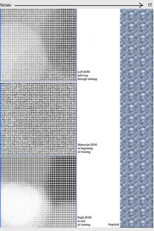
The
striate was modelled using three self-organising networks (SOMs), one
representing neurons that only get information from the left eye, one
representing neurons that only get information from the right eye, and
one representing binocular neurons that get information from both eyes
(Figure 3). Each SOM comprised 900 nodes, where one node represented
a cluster of neurons, and each node had 1600 (40x40) connection weights,
where the connection weights, when seen as a whole for one node, represented
the stimuli for which that node was most likely to “fire”.
The
IT area was modelled using a Hopfield network, but due to uncertainty
about the test results from the IT, this part of the model will
not be discussed further in the present report.
Thus,
the revised aim of the present study was to investigate the abridged
model of the visual system, exploring what sort of input would rival,
if any, in the striate area of the model, as a preliminary for
a bigger study in which rivalry would be investigated in the whole model.
It was hypothesised that incongruent, simple-shape pictures would rival
in the striate whereas incongruent, complex shapes would not.
No congruent pictures were expected to rival.
Method
Apparatus
The
hybrid neural network was programmed in C++ to allow the authors maximum
flexibility in designing the network, and because such an implementation
would run faster than any off-the-shelf software (Appendix A). Training
and testing of the network was performed on a 2.44 GHz, off-the-shelf
IBM compatible single-processor personal computer with 1 GB of memory.
For
training 40 black and white 50x40 pixel pictures were used, 20 of which
represented simple geometric shapes (e.g., a triangle, a circle, a square),
and 20 of which represented more complex shapes (e.g., a triangle and
a square, a “house”).
For
testing, 160 pairs of 50x40 pixel black and white pictures divided into
8 (23) groups were used (Table 1). Groupings were based on
whether or not the pictures were familiar to the networks (i.e., they
were part of the training set), whether the pictures were simple or
complex, and whether or not the pictures presented to the two “eyes”
were the same picture or different pictures (i.e., rivalry was expected
for the second but not the first condition).
Procedure
Before
training, all weights were assigned pseudo-random1 numbers between 0 and 1. During training, the
40 training pictures were presented to the three SOMs in random order
for 7,000, 10,000, and 30,000 iterations on three consecutive runs.
Out of the 50 horizontal pixels for each of the 40 lines, the 40 leftmost
pixels were input to the left-SOM, the 40 rightmost pixels were input
to the right-SOM, and the 30 pixels in the middle were input to the
binocular-SOM (Figure 4). To make the binocular pictures the same size
as the left and right pictures, five black (0) pixels were padded on
each side of every line (Figure 5). In this way, the network was trained
to expect congruent information to the two “eyes.”
During
testing, the 160 pairs of testing pictures were shown to the three trained
networks (left-SOM, binocular-SOM, and right-SOM). The leftmost part
of the first picture was fed to the left-SOM, the rightmost part of
the second picture was fed to the right-SOM. For the binocular-SOM,
the 30 middle pixels of the two pictures were merged in the following
way. If two corresponding pixels were the same (i.e., either both black
or both white), the pixel was fed as-is to the binocular-SOM. Otherwise,
a random number between the numbers representing black (0) and white
(1) was created2.
In
response to each pair of pictures, the three networks outputted the
Best Matching Unit (BMU): the node that most closely matched the input,
where closeness was measured by Euclidian distance. The Euclidian distance
between the left and the binocular BMU was subsequently calculated,
and the Euclidian distance between the right and the binocular BMU was
calculated. Finally, the absolute difference between these two numbers
was taken; this was called the Rivalry Score (RS). A high RS would mean
that the two “eyes” — the left and the right SOM — were seeing different
things, and were thus “rivalling.”
Results
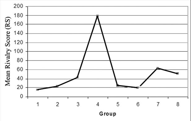
Results were similar for the 7,000, 10,000 and
30,000 iteration trials, and were therefore collated. A
one-way between-subjects ANOVA revealed a main effect of group, F(7,152)
= 4.1862, p < .001. Post-hoc comparisons using the Tukey HSD
test revealed that incongruent pictures of unfamiliar, simple pictures
(group 4) scored higher on the RS than all congruent pictures (groups
1, 2, 5, 6, p < .05 for all groups) (Figure 6). Group 4 pictures
also scored higher on the RS than incongruent, familiar, simple pictures
(group 3, p < .05), hence the unfamiliarity of the pictures
seemed to add to the score.
Discussion
The
results supported the hypothesis that incongruent, simple shapes would
rival in the model striate, whereas complex shapes would not.
Also, as expected, no congruent pictures rivalled. These results are
consistent with the broader hypothesis that rivalry will be found at
several stages (Blake, 1995) throughout the information processing stream,
and that more complex stimuli will show more evidence of rivalry higher
up in the processing "hierarchy," even though it remains to
be seen what will happen further up the processing stream in a fuller
version of the model.
The
raw Rivalry Score (RS) used in the present study cannot signal whether
or not rivalry “actually” occurred in the model. There was no threshold
level, over which rivalry could be said to occur, and there was no final
judge to decide whether or not rivalry had really occurred; all that
could be stated was that the RS was significantly higher for
some groups of pictures than for others. This admittedly vague definition
as to whether or not the model displays rivalry mirrors Blake’s concern
that it is "an oversimplification to speak of rivalry 'occurring'
at any one particular neural locus" (2001, p. 32). Thus, rather
than picking a relatively arbitrary cut-off point for what constituted
rivalry in the model, it was decided to look for traces or evidence
of rivalry.
It
is worth while tracing what is happening in the model striate at depth,
to gain an understanding of what is actually happening in the model,
and to point out a plausible different interpretation of the results.
As described above, the three SOMs had 900 nodes (or neurons) each and
each node could represent a whole 40x40 input picture by its weights.
Given that the training set only consisted of 40 different pictures,
it is not only conceivable, but quite likely, that the SOMs never abstracted
features from the inputs, but instead came to have nodes that represented
every training picture perfectly. Thus, at testing time, when the left
and right SOMs were asked to return the node that matched best with
the test input (the BMU), they returned, in the case of familiar pictures,
exactly the same picture as they were given, since this had already
been perfectly learned (and a picture will always have the least Euclidian
distance from itself, i.e., 0).
In
the case of congruent pictures, the left and right pictures would be
almost3 the same and the binocular picture would have
approximately the same 30 middle pixels, plus five black pixels on both
sides for every line. Thus, the Euclidian distance between the left
and the binocular picture would mostly come from the padding on both
sides of the binocular picture; and likewise for the distance between
the binocular and the right picture. Since the left and right pictures
in this case are almost identical, the distance left – binocular and
the distance right – binocular should be approximately the same, and
the RS would thus be near zero, i.e., no rivalry. It is interesting
to note that the binocular-SOM could act as a sort of judge: if the
left and right pictures are different, then the picture with the least
Euclidian distance to the binocular picture could be seen as the dominant
at a particular point in time. (Time is not incorporated into the present
model.)
In
the case of incongruent pictures then, the left-BMU and the right-BMU
would be the two different test pictures themselves (minus the missing
left or right edge). The binocular-BMU would be the node that matched
most closely with a picture comprising of the left test picture on the
left side and the right test picture on the right side, and random pixels
in the middle (except where the BMUs are overlapping by chance). This
would be a node on the binocular self-organising map somewhere between
the nodes representing the left input and the right input. More specifically,
this node would probably be about halfway between the left-representing
and the right-representing node4. It is not obvious then, why RS should be high
under this condition. The right side of the binocular BMU should be
as different from the left BMU as the left side of the binocular BMU
from the right BMU, approximately. In other words, the difference between
the left BMU and the binocular BMU should be fairly high, and the distance
between the right BMU and the binocular BMU should be fairly high, but
these two distances should be approximately the same, cancelling each
other out and giving a RS near 0. This line of reasoning suggests that
RS might not be as good a measure of rivalry as initially thought. The
results of the present study could then be explained as follows. The
model behaves as just outlined for both congruent stimuli and complex
incongruent stimuli, explaining that complex incongruent stimuli (groups
7, 8) did not rival (when RS is the measurement of rivalry) in the striate
in the present study. However, that simple incongruent stimuli did
rival could be due to the way the Euclidian distance is calculated.
Euclidian distance is calculated by comparing the two pictures pixel-by-pixel.
All pixels in the current study would have a value between 0 and 1,
and the Euclidian distance is the accumulated differences between pixels.
Thus, complex pictures would have more pixels that just happened to
match (be near each other value-wise), as drawing-colour in the present
study was white (1) and background colour was black (0). Simple pictures,
on the other hand, would have large stretched of background only broken
by a few pixels of white, and the probability of two white pixels overlapping
(when comparing two pictures) would be quite small, thus, most white
pixels would be counted as a whole 1 difference, and the accumulated
sum of differences would grow quite fast. That incongruent, unfamiliar,
simple pictures (group 4) had higher RS scores than incongruent, familiar,
simple pictures (group 3) seems more difficult to explain; the present
author has yet to figure out what elements of the model causes this
behaviour.
It
might be concluded that even though the model at first glance produced
results quite consistent with the expectations and hypothesis, caution
should be used when interpreting these results. A thorough investigation
of the model has provided an explanation for the results that should
make one highly reluctant to draw any conclusions about the biological
basis of binocular rivalry, based on this particular model.
To
rectify some of the problems mentioned above with the current model,
future researchers might test the current model with fewer neurons (or
nodes) in each SOM, giving the SOMs opportunity to abstract over several
cases. Pictures could be given different background colours so that
simple pictures would not automatically be very different from each
other. Also, other measures than Euclidian distance could be used for
testing, maybe other measures might be better for detecting rivalry.
Further studies might extend the computer implementation to comprise
the unabridged model; fewer neurons in each layer (compared to the number
of training pictures), but more layers would render the implementation
more biologically realistic. The assumption (implicit in this study)
that nodes in SOMs can represent whole clusters of neurons without loss
of fidelity should be examined, and if it is found not to hold, the
“fewer neurons in more layers”-strategy could be the solution for this
is as well. An extended model would incorporate time into its structure,
allowing researchers to investigate whether or not the model displays
alternations in visibility of images, which is characteristic for binocular
rivalry in humans. This would also allow the comparison of the model
performance with other data on binocular rivalry reported in the literature.
References
| Blake,
R. (1977). Threshold conditions for binocular rivalry. Journal
of Experimental Psychology: Human Perception and Performance, 3,
pp. 251-257. |
Blake, R.,
(1989). A neural theory of binocular rivalry. Psychological Review,
96, pp.145-167.
| Blake,
R. (1995). Psychoanatomical strategies for studying human vision.
In Early vision and beyond, T. Papathomas, C. Chubb, E. Kowler,
A. Gorea (Eds.). MIT Press, Cambridge. |
Blake,
R. (2001). Primer
on binocular rivalry, including controversial issues. Brain and
Mind, 2, pp. 5-38.
Blake,
R., Westendorf, D., & Overton, R. (1980). What is suppressed during
binocular rivalry? Perception, 9, pp. 223-231.
Dutour, E. F. (1760). Discussion d'une
question d'optique [Discussion on a question of optics]. l'Académie
des Sciences. Mémoires de Mathématique et de physique présentés par
Divers Savants, 3, pp.514-530.
Fox,
R., & Rasche, F. (1969). Binocular rivalry and reciprocal inhibition.
Perception and Psychophysics, 5, pp. 215-217.
Kohonen,
T. (1995). Self-organizing maps. Berlin ; New York: Springer. |
Lee,
S. H., & Blake, R. (1999). Rival ideas about binocular rivalry.
Vision Research, 39, pp. 1447-1454.
Leopold,
D. A., & Logothetis, N. K (1996). Activity changes in early visual
cortex reflect monkeys' percepts during binocular rivalry. Nature,
379, p. 549.
Levelt,
W. (1965). On binocular rivalry. Soesterberg, The Netherlands,
Institute for Perception RVO-TNO.
Liu,
L. Tyler, C, & Schor, C. (1992). Failure of rivalry at low contrast:
Evidence of a suprathreshold binocular summation. Nature, 379,
pp. 549-554.
Logothetis,
N. K., Leopold, D. A., & Sheinberg, D. L. (1996). What is rivalling
during binocular rivalry? Nature, 380, pp. 621-624.
Mitchison,
G. J., & Swindale, N. V. (1999). Can Hebbian volume learning explain
discontinuities in cortical maps? Neural Computing, 11(7), 1519-1526.
O'Shea, R.
P. (1999). Translation
of Dutour (1760) [On-line]. Available: http://psy.otago.ac.nz/r_oshea/dutour60.html
Riesenhuber,
M., Bauer, H., Brockmann, D., & Geisel, T. (1998). Breaking rotational
symmetry in a self-organizing map model for orientation map development.
Neural Computing, 10(3), 717-730.
Sheinberg,
D. L., & Logothetis, N. K. (1997). The role of temporal cortical
areas in perceptual organization. Proceedings of the National Academy
of Science, USA, 94, pp. 3408-3413.
Wiemer,
J., Burwick, T., & von Seelen, W. (2000). Self-organizing maps for
visual feature representation based on natural binocular stimuli. Biological
Cybernetics, 82(2), 97-110.
Wolf, F., Bauer, H. U.,
Pawelzik, K., & Geisel, T. (1996). Organization of the visual cortex.
Nature, 382(6589), 306-307.
Appendix A: Code
Several
version of the MSVC++ project including C++ code can be downloaded from
http://www.stenmorten.com/CogSci/Code.htm
. The latest version is ftp://ftp.stenmorten.f2s.com/www.stenmorten.f2s.com/KmZB/Brain030903_2114.zip
Footnotes
1.
For the present purposes, the pseudo-random numbers created by the algorithm
in C++ are “random enough”, that is, they have the needed mathematical
properties, and hence they will be referred to as random from here on.
2.
Taking the average of the two numbers would be presupposing that opposing
information is merged in the early parts of the visual processing system,
something that is definitively not supported by the empirical evidence;
anyway, in the present model, the average would always be (1+0)/2 =0.5.
ANDing the numbers together would always render the pixel invisible
(0) – effectively saying that if one eye cannot see it, then the other
eye cannot see it either (so if the model “closed one eye”, it would
be blind). Conversely, ORing the numbers would always render the pixel
on (or 1).
3.
The pictures are not exactly the same as the test inputs, because the
left-SOM only learned the 40 leftmost of the full 50 pixels of every
training picture, and the right-SOM only learned the 40 rightmost pixels.
4.
This is because of the way the SOMs learn during training. When a training
picture is presented to the SOM, the BMU is found and the Euclidian
distance between the training picture and the BMU is calculated. Then,
in a circular fashion, the nodes around the BMU are all updated to be
more like the training picture, with the BMU itself being made most
like the training picture and the nodes around it less so, the training
factor decreasing as the distance between the BMU and the node to be
trained increases.
Table
1
Test
picture groups
-------------------------------------------------------------------------
Group Congruent Familiar
Simple
-------------------------------------------------------------------------
1 v v
v
2 v v
3
v v
4
v
5 v v
6 v
7
v
8
-------------------------------------------------------------------------
Figure Captions
Figure 1. High-level view of the model. Thick
arrows indicate main flow of information. Arrows from left to right
represent information flowing "up" in the processing "hierarchy",
and is assumed to get more complex as it goes. Arrows from right to
left indicate recurrent connections. i sends information to both V1
and V+, and receives recurrent connections from both V1 and IT. Each
layer is a separate kind of network corresponding to the type of network
found in wetware.
Figure 2. The eyes/LGN; here shown with i = 2*(3) for simplicity. This structure
consists of approximately 50% binocular neurons. Sub-layer 1 is monocular;
whereas about half of the neurons of sub-layer 2 to m are binocular.
Information flows from left to right. Only excitatory connections are
shown.
Figure
3. The abridged
network. Three self-organising maps (SOMs) representing neurons of the
left eye, neurons of the right eye, and binocular neurons, feed into
the Hopfield network, representing the inferotemporal (IT) cortex.
Figure
4. Training
input. The left SOM, the right SOM, and the binocular SOM are trained
on different parts of the same pictures.
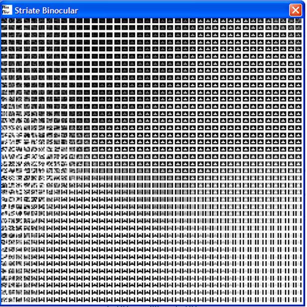
Figure
5. The binocular
SOM late in training. Every trained node in the binocular SOM has black
(0) padding on both sides.
Figure
6. Mean Rivalry Score (RS) for each
group of stimuli.

Figure 1.
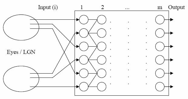
Figure 2.
Figure
3.
Figure
4.
Figure
5.
Figure
6.